Optimal Transport Models
Optimal Transport models are useful tools in evaluating the potential effeciency of flat-rate mass transit systems where full trips are not recorded (like the NYC subway system, but unlike the San Francisco BART system).
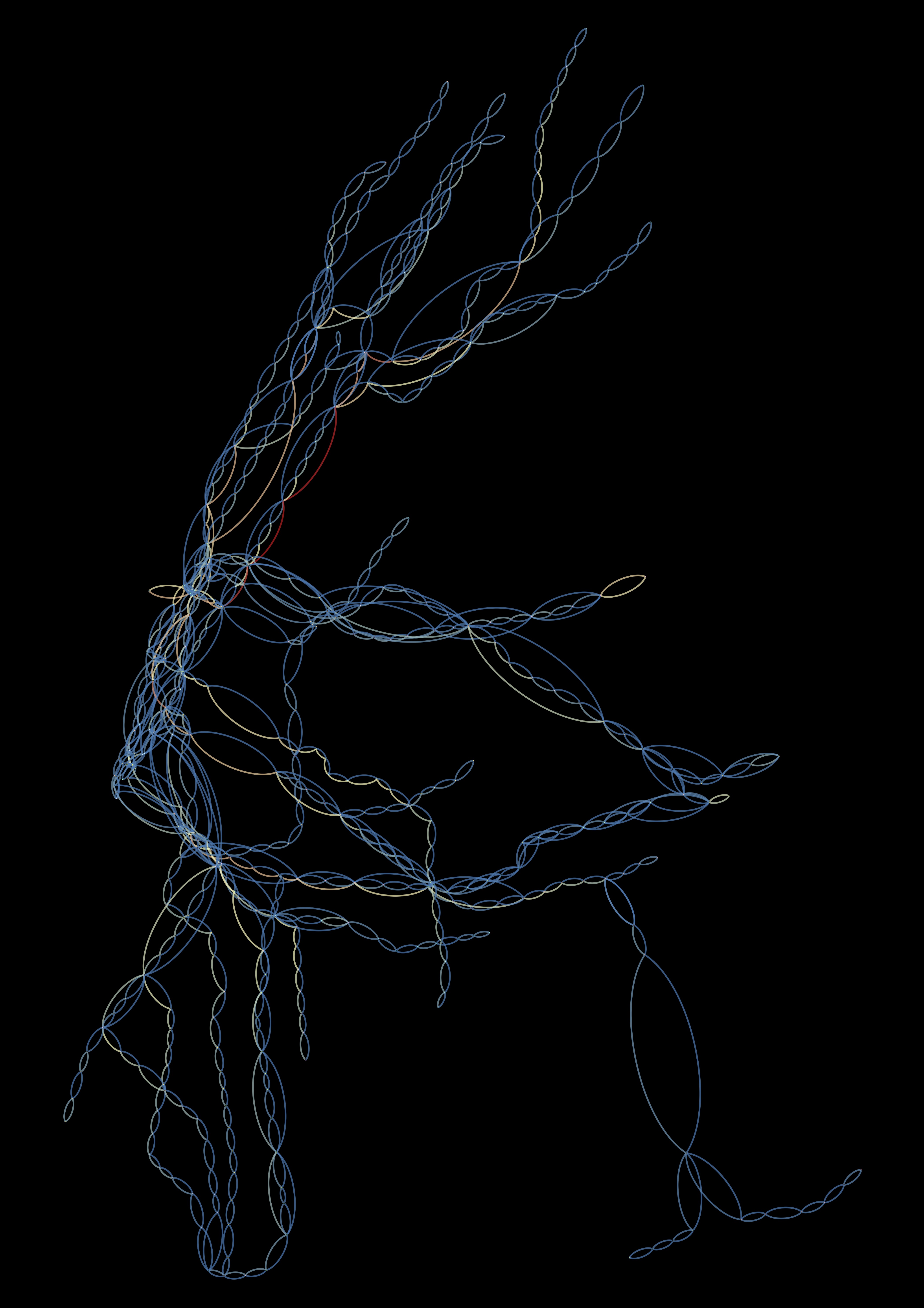
By assuming that commuters strive to take the routes which minimize the total system transit time while conforming to the station entrance and exit data we can establish a lower bound for the aggregate effeciency of the whole system. We can also look at which links in the system are most heavily used given these optimality assumptions. Below is a gephi rendering of the cost minimizing flows (the vector $\mathbf{\Pi}$ defined in the next section) accross track segments in the nyc subway sys.

Model Definitions
A typical (simplified) setting for optimal transport models which you might see described in an economics textbook is a trading network for a single resource with a set of supply and demand nodes $\mathcal{X}$ (cities), and a set of directed arcs $\mathcal{A}$ (roads) between them. The primal and dual problems are ones of transport cost minimization (optimizing trading flow rates over all conduits) and profit maximization (optimizing prices for goods at each city). An $\vert \mathcal{A} \vert \times \vert \mathcal{X} \vert$ edge-node matrix $\nabla$ defines the topological structure of this system. For each $x \in \mathcal{X}$ and $a \in \mathcal{A}$, we have and entry in $\nabla$:
$\nabla$: The gradient matrix; a useful representation of the network topology which allows us to succinctly define the relevant optimization problems using vector notation.
$\mathbf{\Pi}$: The flow vector; a set of real values representing the flow of goods between each city in a trading network, or the flow of commuters between each station in a transit network. The model allows us to estimate the values of this vector.
$\mathbf{c}$: The cost vector; a set of real values representing the cost of traveling between each city in a trading network, or the travel costs for commuters between each station in a transit network (i.e. travel times). We must populate this vector with reasonable values supported by some data before running the optimization.
$\mathbf{\Phi}$: The prices vector; a set of real values representing the ``price'' at each city or station. This can be thought of a loose proxy for real estate prices, however we are more concerned with estimating the flow for transit systems.
$\mathbf{n}$: The supply vector; a set of real values representing how many goods are produced or consumed at each city (must be one or the other), or the net contribution of commuters by each station in a transit network.
$$ \nabla_{ax} = \begin{cases} +1, & \text{if $a$ is an in-edge of $x$}\ \\ -1, & \text{if $a$ is an out-edge of $x$}\ \\ 0, & \text{otherwise} \end{cases} $$
Note that $\nabla$ is sparse by definition, containing only two entries per row ($1$ and $-1$ for each edge). The production (if positive) or demand (if negative) of each city is described by the vector $\mathsf{\mathbf{n}}$, with one entry for each city. Additionally we describe the costs associated with each arc as a vector of edge weights $\mathsf{\mathbf{c}}$. As mentioned, the primal and dual problems can be used to infer \textit{flows} over edges $\mathbf{\Pi}$, by solving
\begin{equation} \min_{\mathbf{\Pi}_a \geq 0, \ \forall a \in \mathcal{A}} \mathbf{\Pi} \cdot \mathsf{\mathbf{c}}\ , \ \ \ \text{subject to} \ \ \ \nabla^\top \cdot \mathbf{\Pi} = \mathbf{n} \end{equation} or $prices$ $\mathbf{\Phi}$ at each city by solving \begin{equation} \max_{\mathbf{\Phi} \in \mathbb{R}^\mathcal{X}} \mathbf{\Phi} \cdot \mathsf{\mathbf{n}}\ , \ \ \ \text{subject to} \ \ \ \nabla \cdot \mathbf{\Phi} \leq \mathbf{c} \end{equation}
We can use additional constraints to better fit the real world entrance/exit data at hand. For example, the above model only takes into account each
Feasibility Conditions
In order for the above optimization problems to be feasible, i.e. to guarantee the existence of $\mathbf{\Pi}$ and $\mathbf{\Phi}$ given the constraints, a few criteria must be met for the network:
$Balancedness$: Nodes are defined as supply or demand nodes based on the sign of their entries in $\mathbf{n}$, and we assume that exactly all of the supply is eventually consumed by the demand nodes, i.e. $$\sum_{x \in \mathcal{X}} n_x = 0$$
$Connectedness$: The set of supply nodes $\mathbf{n}_+, \subset \mathbf{n}$ and demand nodes $\mathbf{n}_- \subset \mathbf{n}$ are such that $\mathbf{n}_+$ is strongly connected to $\mathbf{n}_-$, i.e. there is a path from every $n_i \in \mathbf{n}_+$ to every $n_j \in \mathbf{n}_-$.
$No$ $Profitable$ $Loop$ / $Zero-Arbitrage$: There are no arbitrage opportunities with negative cost loops. We can enforce this easily by setting $$c_a \geq 0, \ \forall c_a \in \mathbf{c} $$
These are the basic components of the optimal transport problem defined on trading networks. Various modifications must be made to better accommodate the commuter transit setting.